Introduction to Trefftz-DG

We give a short introduction to Trefftz-DG methods for the model problem of the Laplace equation.

\[\begin{split}\newcommand{\Th}{{\mathcal{T}_h}} \newcommand{\Fh}{\mathcal{F}_h} \newcommand{\dom}{\Omega} \newcommand{\jump}[1]{[\![ #1 ]\!]} \newcommand{\tjump}[1]{[\![{#1} ]\!]_\tau} \newcommand{\avg}[1]{\{\!\!\{#1\}\!\!\}} \newcommand{\nx}{n_\mathbf{x}} \begin{align*} \begin{split} \begin{cases} -\Delta u = 0 &\text{ in } \Omega, \\ u=g &\text{ on } \partial \Omega, \end{cases} \end{split} \end{align*}\end{split}\]

Harmonic polynomials

For an element \(K\) in out mesh \(\Th\) we define the local Trefftz space as

\[\begin{align*} \begin{split} \mathbb{T}^p(K):=\big\{ f\in\mathbb{P}^p(K) \mid \Delta f = 0 \big\}, \qquad p\in \mathbb{N}. \end{split} \end{align*}\]

For the Laplace problem the Trefftz space is given by harmonic polynomials, e.g. for polynomials of order 3 in two dimensions the space is given by

\[\begin{align*} \begin{split} \mathbb{T}^3(K)=\text{span}\{1,x,y,xy,x^2-y^2,x^3-3y^2x,y^3-3x^2y\} \end{split} \end{align*}\]

The local degrees of freedom are reduced from the dimension of the full polynomials, given by \(\big(\begin{smallmatrix}p+n\\p\end{smallmatrix}\big)\), to

\[\begin{split}\begin{align*} \begin{split} \dim\mathbb{T}^p(K)=\begin{cases} 2 & n=1\\ 2p+1 & n=2\\ (p+1)^2 & n=3\end{cases}. \end{split} \end{align*}\end{split}\]

Numerical treatment

The IP-DG method for the Laplace equation is given by

\[\begin{split}\begin{align}\label{eq:dglap} \begin{split} a_h(u,v) &= \int_\dom \nabla u\nabla v\ dV -\int_{\Fh^\text{int}}\left(\avg{\nabla u}\jump{v}+\avg{\nabla v}\jump{u} - \frac{\alpha p^2}{h}\jump{u}\jump{v} \right) dS \\ &\qquad -\int_{\Fh^\text{bnd}}\left(\nx\cdot\nabla u v+\nx\cdot\nabla v u-\frac{\alpha p^2}{h} u v \right) dS\\ \ell(v) &= \int_{\Fh^\text{bnd}}\left(\frac{\alpha p^2}{h} gv -\nx\cdot\nabla vg\right) dS. \end{split} \end{align}\end{split}\]

where \(h\) is the mesh size, \(p\) is the polynomial degree and \(\alpha>0\).

For a given mesh we construct the Trefftz finite element space as

\[\begin{align*} \begin{split} \mathbb{T}^p(\Th):=\prod_{K\in\Th} \mathbb{T}^p(K) \end{split} \end{align*}\]

in NGSolve this is done by

mesh = Mesh(unit_square.GenerateMesh(maxh=.5))
trefftzfespace(mesh,order=p,eq="laplace",dgjumps=True)

We will compare the approximation properties of the Trefftz space with the space of (all) piecewise polynomials. In NGSolve

L2(mesh,order=p,dgjumps=True)

The numerical results for the Trefftz space are plotted in solid lines, while the results for the full polynomial space are the dashed lines. We show the convergence rates with respect to polynomial degree \(p\) and mesh size \(h\). In the Figure on the left we show the error compared to the global number of degrees of freedom for varying \(p\). In the Figure on the right we show the error with respect to \(h\).

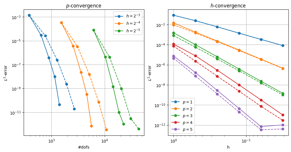
The Trefftz space shows optimal rate of convergence, using fewer degrees of freedom. As an exact solution we used

\[u(x,y) = \exp(x)\sin(y) \quad \text{in} \quad [0,1]^2.\]

from ngsolve.webgui import Draw
mesh = Mesh(unit_square.GenerateMesh(maxh=0.3))
fes = trefftzfespace(mesh,order=5,eq="laplace",dgjumps=True)
(a,f) = lap_problem(fes)
gfu = GridFunction(fes)
gfu.vec.data = a.mat.Inverse(inverse='sparsecholesky') * f.vec
Draw(gfu)

BaseWebGuiScene

How to get started?

If you want to see more implementations using Trefftz-DG methods or use an already implemented Trefftz space, have a look at the notebooks and the documentation.
If you are looking to implement a (polynomial) Trefftz space, a good starting point is to have a look at trefftzspace.hpp. For Trefftz spaces based on plane waves check out planewavefe.hpp.
Before undertaking the implementation of a new Trefftz space in C++, or especially if your PDE does not have a easy-to-construct Trefftz space, consider checking out the embedded Trefftz method.

If you are implementing a new method using NGSTrefftz consider contributing.