Laplace

We are looking to solve

\[\begin{split}\begin{align*} \begin{split} \begin{cases} -\Delta u = 0 &\text{ in } \Omega, \\ u=g &\text{ on } \partial \Omega, \end{cases} \end{split} \end{align*}\end{split}\]

using a Trefftz-DG formulation

from ngsolve import *
from ngstrefftz import *
from netgen.occ import *

Constructing a Trefftz space

A Trefftz space for the Laplace problem is given by the harmonic functions that locally fulfil

\[\begin{align*} \begin{split} \mathbb{T}^p(K):=\big\{ f\in\mathbb{P}^p(K) \mid \Delta f = 0 \big\}, \qquad p\in \mathbb{N}. \end{split} \end{align*}\]

We can construct it in NGSolve like so:

mesh = Mesh(unit_square.GenerateMesh(maxh=.3))
fes = trefftzfespace(mesh,order=7,eq="laplace")

Using the eq key word one needs to tell the Trefftz space the operator for which to construct Trefftz functions.

To get an overview on the implemented Trefftz functions see

trefftzfespace?

We will test against an exact solution given by

exact = exp(x)*sin(y)
bndc = exact

A suiteable DG method is given by

\[\begin{split}\newcommand{\Th}{{\mathcal{T}_h}} \newcommand{\Fh}{\mathcal{F}_h} \newcommand{\dom}{\Omega} \newcommand{\jump}[1]{[\![ #1 ]\!]} \newcommand{\tjump}[1]{[\![{#1} ]\!]_\tau} \newcommand{\avg}[1]{\{\!\!\{#1\}\!\!\}} \newcommand{\nx}{n_\mathbf{x}} \begin{align}\label{eq:dglap} \begin{split} a_h(u,v) &= \int_\dom \nabla u\nabla v\ dV -\int_{\Fh^\text{int}}\left(\avg{\nabla u}\jump{v}+\avg{\nabla v}\jump{u} - \frac{\alpha p^2}{h}\jump{u}\jump{v} \right) dS \\ &\qquad -\int_{\Fh^\text{bnd}}\left(\nx\cdot\nabla u v+\nx\cdot\nabla v u-\frac{\alpha p^2}{h} u v \right) dS\\ \ell(v) &= \int_{\Fh^\text{bnd}}\left(\frac{\alpha p^2}{h} gv -\nx\cdot\nabla vg\right) dS. \end{split} \end{align}\end{split}\]

def dglap(fes,bndc):
    mesh = fes.mesh
    order = fes.globalorder
    alpha = 4
    n = specialcf.normal(mesh.dim)
    h = specialcf.mesh_size
    u = fes.TrialFunction()
    v = fes.TestFunction()

    jump_u = (u-u.Other())*n
    jump_v = (v-v.Other())*n
    mean_dudn = 0.5 * (grad(u)+grad(u.Other()))
    mean_dvdn = 0.5 * (grad(v)+grad(v.Other()))

    a = BilinearForm(fes,symmetric=True)
    a += grad(u)*grad(v) * dx \
        +alpha*order**2/h*jump_u*jump_v * dx(skeleton=True) \
        +(-mean_dudn*jump_v-mean_dvdn*jump_u) * dx(skeleton=True) \
        +alpha*order**2/h*u*v * ds(skeleton=True) \
        +(-n*grad(u)*v-n*grad(v)*u)* ds(skeleton=True)

    f = LinearForm(fes)
    f += alpha*order**2/h*bndc*v * ds(skeleton=True) \
         +(-n*grad(v)*bndc)* ds(skeleton=True)

    with TaskManager():
        a.Assemble()
        f.Assemble()
    return a,f

a,f = dglap(fes,bndc)
gfu = GridFunction(fes)
with TaskManager():
    gfu.vec.data = a.mat.Inverse(inverse='sparsecholesky') * f.vec
error = sqrt(Integrate((gfu-exact)**2, mesh))
print("trefftz",error)

trefftz 3.935899697867962e-12

from ngsolve.webgui import Draw
Draw(gfu)

BaseWebGuiScene

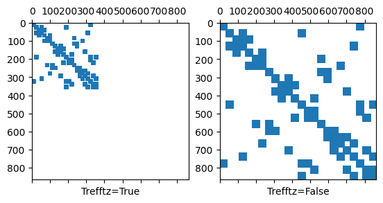
Comparison of the sparsity pattern

We compare the sparsity pattern to the one of the full polynomial \(\texttt{L2}\) space

import scipy.sparse as sp
import numpy as np
import matplotlib.pylab as plt
a2,_ = dglap(L2(mesh,order=7,dgjumps=True),bndc)

A1 = sp.csr_matrix(a.mat.CSR())
A2 = sp.csr_matrix(a2.mat.CSR())
fig = plt.figure(); ax1 = fig.add_subplot(121); ax2 = fig.add_subplot(122)
ax1.set_xlabel("Trefftz=True"); ax1.spy(A1,markersize=1); ax1.set(ylim=(a2.mat.height,0),xlim=(0,a2.mat.width))
ax2.set_xlabel("Trefftz=False"); ax2.spy(A2,markersize=1)

<matplotlib.lines.Line2D at 0x7f757413cf10>